Note
Go to the end to download the full example code.
Price Optimization
Develop a data science pipeline for pricing and distribution of avocados to maximize revenue.
Note
This example is adapted from the example in Gurobi’s modeling examples How Much Is Too Much? Avocado Pricing and Supply Using Mathematical Optimization.
The main difference is that it uses Scikit-learn for the
regression model and Gurobi Machine Learning to formulate the regression
in a Gurobi model.
But it also differs in that it uses Matrix variables and that the interactive part of the notebook is skipped. Please refer to the original example for this.
This example illustrates in particular how to use categorical variables in a regression.
If you are already familiar with the example from the other notebook, you can jump directly to building the regression model and then to formulating the optimization problem.
A Food Network article from March 2017 declared, “Avocado unseats banana as America’s top fruit import.” This declaration is incomplete and debatable for reasons other than whether avocado is a fruit. Avocados are expensive.
As a supplier, setting an appropriate avocado price requires a delicate trade-off. Set it too high and you lose customers. Set it too low, and you won’t make a profit. Equipped with good data, the avocado pricing and supply problem is ripe with opportunities for demonstrating the power of optimization and data science.
They say when life gives you avocados, make guacamole. Just like the perfect guacamole needs the right blend of onion, lemon and spices, finding an optimal avocado price needs the right blend of descriptive, predictive and prescriptive analytics.
This notebook walks through a decision-making pipeline that culminates in a mathematical optimization model. There are three stages:
First, understand the dataset and infer the relationships between categories such as the sales, price, region, and seasonal trends.
Second, build a prediction model that predicts the demand for avocados as a function of price, region, year and the seasonality.
Third, design an optimization problem that sets the optimal price and supply quantity to maximize the net revenue while incorporating costs for wastage and transportation.
Load the Packages and the Datasets
We use real sales data provided by the Hass Avocado Board (HAB), whose aim is to “make avocados America’s most popular fruit”. This dataset contains consolidated information on several years’ worth of market prices and sales of avocados.
We will now load the following packages for analyzing and visualizing the data.
import gurobipy as gp
import gurobipy_pandas as gppd
import matplotlib.pyplot as plt
import numpy as np
import pandas as pd
import seaborn as sns
from sklearn.compose import make_column_transformer
from sklearn.linear_model import LinearRegression
from sklearn.metrics import r2_score
from sklearn.model_selection import train_test_split
from sklearn.pipeline import make_pipeline
from sklearn.preprocessing import OneHotEncoder, StandardScaler

from gurobi_ml import add_predictor_constr
The dataset from HAB contains sales data for the years 2019-2022. This data is augmented by a previous download from HAB available on Kaggle with sales for the years 2015-2018.
Each row in the dataset is the weekly number of avocados sold and the weekly average price of an avocado categorized by region and type of avocado. There are two types of avocados: conventional and organic. In this notebook, we will only consider the conventional avocados. There are eight large regions, namely the Great Lakes, Midsouth, North East, Northern New England, South Central, South East, West and Plains.
Now, load the data and store into a Pandas dataframe.
data_url = "https://raw.githubusercontent.com/Gurobi/modeling-examples/master/price_optimization/"
avocado = pd.read_csv(
    data_url + "HABdata_2019_2022.csv"
)  # dataset downloaded directly from HAB
avocado_old = pd.read_csv(
    data_url + "kaggledata_till2018.csv"
)  # dataset downloaded from Kaggle

# The date is in different formats in the two data sets and
# need to be converted separately
avocado["date"] = pd.to_datetime(avocado["date"], format="%m/%d/%y %H:%M")
avocado_old["date"] = pd.to_datetime(avocado_old["date"], format="%m/%d/%y")

# Concatenate the two notebooks
avocado = pd.concat([avocado, avocado_old])
avocado
Prepare the Dataset
We will now prepare the data for making sales predictions. Add new columns to the dataframe for the year and seasonality. Let each year from 2015 through 2022 be given an index from 0 through 7 in the increasing order of the year. We will define the peak season to be the months of February through July. These months are set based on visual inspection of the trends, but you can try setting other months.
# Add the index for each year from 2015 through 2022
avocado["year"] = pd.DatetimeIndex(avocado["date"]).year
avocado = avocado.sort_values(by="date")

# Define the peak season
avocado["month"] = pd.DatetimeIndex(avocado["date"]).month
peak_months = range(2, 8)  # <--------- Set the months for the "peak season"


def peak_season(row):
    return 1 if int(row["month"]) in peak_months else 0


avocado["peak"] = avocado.apply(lambda row: peak_season(row), axis=1)

# Scale the number of avocados to millions
avocado["units_sold"] = avocado["units_sold"] / 1000000

# Select only conventional avocados
avocado = avocado[avocado["type"] == "Conventional"]

avocado = avocado[
    ["date", "units_sold", "price", "region", "year", "month", "peak"]
].reset_index(drop=True)

avocado
Part 1: Observe Trends in the Data
Now, we will infer sales trends in time and seasonality. For simplicity, let’s proceed with data from the United States as a whole.
df_Total_US = avocado[avocado["region"] == "Total_US"]
Sales Over the Years
fig, axes = plt.subplots(nrows=1, ncols=1, figsize=(10, 5))

mean = df_Total_US.groupby("year")["units_sold"].mean()
std = df_Total_US.groupby("year")["units_sold"].std()
axes.errorbar(mean.index, mean, xerr=0.5, yerr=2 * std, linestyle="")
axes.set_ylabel("Units Sold (millions)")
axes.set_xlabel("Year")

fig.tight_layout()
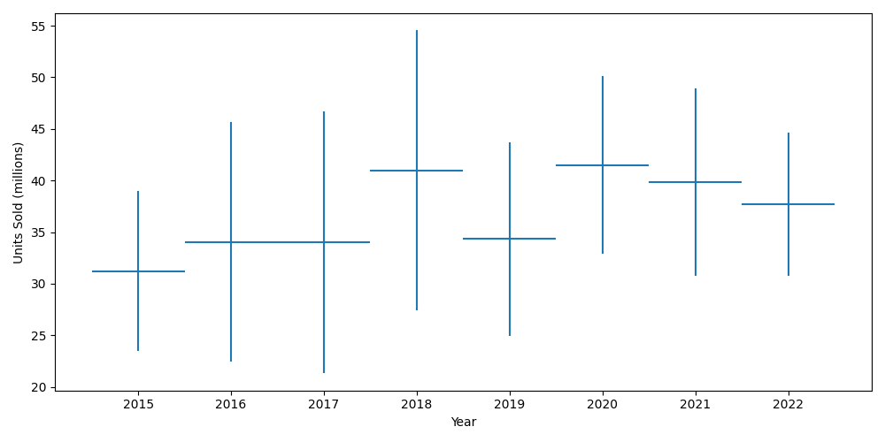
We can see that the sales generally increased over the years, albeit marginally. The dip in 2019 is the effect of the well-documented 2019 avocado shortage that led to avocados nearly doubling in price.
Seasonality
We will now see the sales trends within a year.
fig, axes = plt.subplots(nrows=1, ncols=1, figsize=(10, 5))

mean = df_Total_US.groupby("month")["units_sold"].mean()
std = df_Total_US.groupby("month")["units_sold"].std()

axes.errorbar(mean.index, mean, xerr=0.5, yerr=2 * std, linestyle="")
axes.set_ylabel("Units Sold (millions)")
axes.set_xlabel("Month")

fig.tight_layout()

plt.xlabel("Month")
axes.set_xticks(range(1, 13))
plt.ylabel("Units sold (millions)")
plt.show()
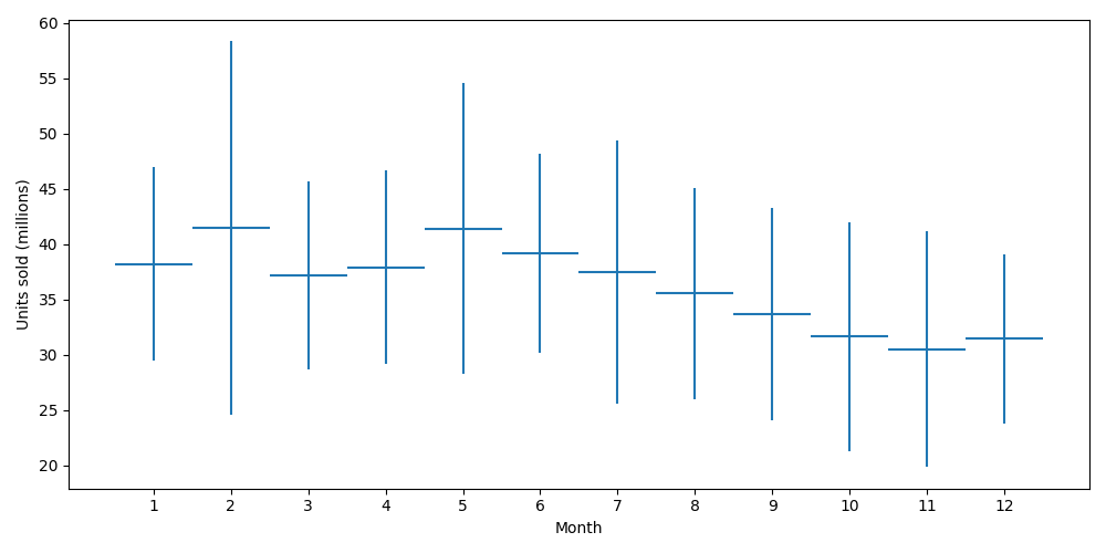
We see a Super Bowl peak in February and a Cinco de Mayo peak in May.
Correlations
Now, we will see how the variables are correlated with each other. The end goal is to predict sales given the price of an avocado, year and seasonality (peak or not).
fig, axes = plt.subplots(nrows=1, ncols=1, figsize=(15, 5))
sns.heatmap(
    df_Total_US[["units_sold", "price", "year", "peak"]].corr(),
    annot=True,
    center=0,
    ax=axes,
)

axes.set_title("Correlations for conventional avocados")
plt.show()
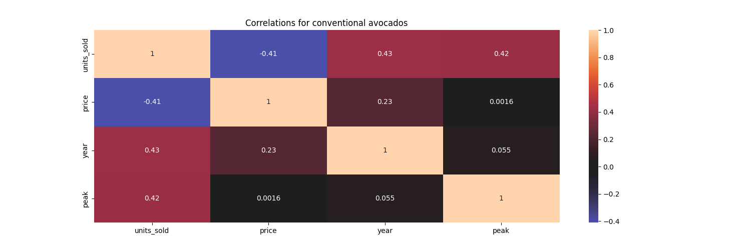
As expected, the sales quantity has a negative correlation with the price per avocado. The sales quantity has a positive correlation with the year and season being a peak season.
Regions
Finally, we will see how the sales differ among the different regions. This will determine the number of avocados that we want to supply to each region.
fig, axes = plt.subplots(nrows=1, ncols=1, figsize=(10, 5))

regions = [
    "Great_Lakes",
    "Midsouth",
    "Northeast",
    "Northern_New_England",
    "SouthCentral",
    "Southeast",
    "West",
    "Plains",
]
df = avocado[avocado.region.isin(regions)]

mean = df.groupby("region")["units_sold"].mean()
std = df.groupby("region")["units_sold"].std()

axes.errorbar(range(len(mean)), mean, xerr=0.5, yerr=2 * std, linestyle="")

fig.tight_layout()

plt.xlabel("Region")
plt.xticks(range(len(mean)), pd.DataFrame(mean)["units_sold"].index, rotation=20)
plt.ylabel("Units sold (millions)")
plt.show()
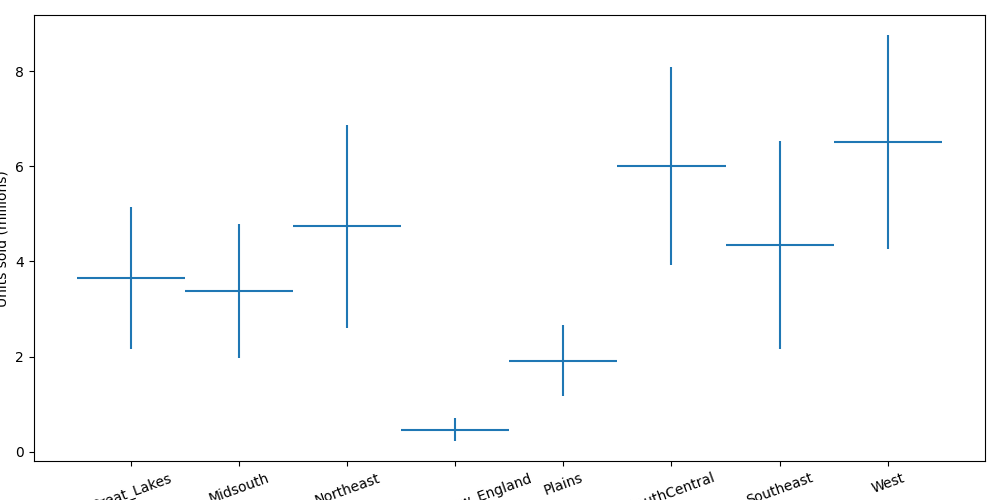
Clearly, west-coasters love avocados.
Part II: Predict the Sales
The trends observed in Part I motivate us to construct a prediction model for sales using the independent variables- price, year, region and seasonality. Henceforth, the sales quantity will be referred to as the predicted demand.
To validate the regression model, we will randomly split the dataset
into \(80\%\) training and \(20\%\) testing data and learn the
weights using Scikit-learn.
Note that the region is a categorical variable.
To apply a linear regression, we need to transform those variable using
an encoding. Here we use Scikit Learn OneHotEncoder. We also use a
standard scaler for prices and year index. All those transformations are
combined with a Column Transformer built using
make_column_transformer.
feat_transform = make_column_transformer(
    (OneHotEncoder(drop="first"), ["region"]),
    (StandardScaler(), ["price", "year"]),
    ("passthrough", ["peak"]),
    verbose_feature_names_out=False,
    remainder="drop",
)
The regression model is a pipeline consisting of the
Column Transformer we just defined and a Linear Regression.
Define it and train it.
lin_reg = make_pipeline(feat_transform, LinearRegression())
lin_reg.fit(X_train, y_train)

# Get R^2 from test data
y_pred = lin_reg.predict(X_test)
print(f"The R^2 value in the test set is {r2_score(y_test, y_pred)}")
The R^2 value in the test set is 0.8982069358257863
We can observe a good \(R^2\) value in the test set. We will now train the fit the weights to the full dataset.
lin_reg.fit(X, y)

y_pred_full = lin_reg.predict(X)
print(f"The R^2 value in the full dataset is {r2_score(y, y_pred_full)}")
The R^2 value in the full dataset is 0.9066729322212482
Part III: Optimize for Price and Supply of Avocados
Knowing how the price of an avocado affects the demand, how can we set the optimal avocado price? We don’t want to set the price too high, since that could drive demand and sales down. At the same time, setting the price too low could be suboptimal when maximizing revenue. So what is the sweet spot?
On the distribution logistics, we want to make sure that there are enough avocados across the regions. We can address these considerations in a mathematical optimization model. An optimization model finds the best solution according to an objective function such that the solution satisfies a set of constraints. Here, a solution is expressed as a vector of real values or integer values called decision variables. Constraints are a set of equations or inequalities written as a function of the decision variables.
At the start of each week, assume that the total number of available products is finite. This quantity needs to be distributed to the various regions while maximizing net revenue. So there are two key decisions - the price of an avocado in each region, and the number of avocados allocated to each region.
Let us now define some input parameters and notations used for creating the model. The subscript \(r\) will be used to denote each region.
Input Parameters
\(R\): set of regions,
\(d(p,r)\): predicted demand in region \(r\in R\) when the avocado per product is \(p\),
\(B\): available avocados to be distributed across the regions,
\(c_{waste}\): cost (\(\$\)) per wasted avocado,
\(c^r_{transport}\): cost (\(\$\)) of transporting a avocado to region \(r \in R\),
\(a^r_{min},a^r_{max}\): minimum and maximum price (\(\$\)) per avocado for reigon \(r \in R\),
\(b^r_{min},b^r_{max}\): minimum and maximum number of avocados allocated to region \(r \in R\),
The following code loads the Gurobi python package and initiates the optimization model. The value of \(B\) is set to \(30\) million avocados, which is close to the average weekly supply value from the data. For illustration, let us consider the peak season of 2021. The cost of wasting an avocado is set to \(\$0.10\). The cost of transporting an avocado ranges between \(\$0.10\) to \(\$0.50\) based on each region’s distance from the southern border, where the majority of avocado supply comes from. Further, we can set the price of an avocado to not exceed \(\$ 2\) apiece.
# Sets and parameters
B = 30  # total amount ot avocado supply

peak_or_not = 1  # 1 if it is the peak season; 1 if isn't
year = 2022

c_waste = 0.1  # the cost ($) of wasting an avocado

# the cost of transporting an avocado
c_transport = pd.Series(
    {
        "Great_Lakes": 0.3,
        "Midsouth": 0.1,
        "Northeast": 0.4,
        "Northern_New_England": 0.5,
        "SouthCentral": 0.3,
        "Southeast": 0.2,
        "West": 0.2,
        "Plains": 0.2,
    },
    name="transport_cost",
)

c_transport = c_transport.loc[regions]
# the cost of transporting an avocado

# Get the lower and upper bounds from the dataset for the price and the number of products to be stocked
a_min = 0  # minimum avocado price in each region
a_max = 2  # maximum avocado price in each region

data = pd.concat(
    [
        c_transport,
        df.groupby("region")["units_sold"].min().rename("min_delivery"),
        df.groupby("region")["units_sold"].max().rename("max_delivery"),
    ],
    axis=1,
)

data
Decision Variables
Let us now define the decision variables. In our model, we want to store the price and number of avocados allocated to each region. We also want variables that track how many avocados are predicted to be sold and how many are predicted to be wasted. The following notation is used to model these decision variables.
\(p\) the price of an avocado (\(\$\)) in each region,
\(x\) the number of avocados supplied to each region,
\(s\) the predicted number of avocados sold in each region,
\(w\) the predicted number of avocados wasted in each region.
\(d\) the predicted demand in each region.
All those variables are created using gurobipy-pandas, with the function
gppd.add_vars they are given the same index as the data
dataframe.
m = gp.Model("Avocado_Price_Allocation")

p = gppd.add_vars(m, data, name="price", lb=a_min, ub=a_max)
x = gppd.add_vars(m, data, name="x", lb="min_delivery", ub="max_delivery")
s = gppd.add_vars(
    m, data, name="s"
)  # predicted amount of sales in each region for the given price).
w = gppd.add_vars(m, data, name="w")  # excess wasteage in each region).
d = gppd.add_vars(
    m, data, lb=-gp.GRB.INFINITY, name="demand"
)  # Add variables for the regression

m.update()

# Display one of the variables
p
Great_Lakes                      <gurobi.Var price[Great_Lakes]>
Midsouth                            <gurobi.Var price[Midsouth]>
Northeast                          <gurobi.Var price[Northeast]>
Northern_New_England    <gurobi.Var price[Northern_New_England]>
SouthCentral                    <gurobi.Var price[SouthCentral]>
Southeast                          <gurobi.Var price[Southeast]>
West                                    <gurobi.Var price[West]>
Plains                                <gurobi.Var price[Plains]>
Name: price, dtype: object
Set the Objective
Next, we will define the objective function: we want to maximize the net revenue. The revenue from sales in each region is calculated by the price of an avocado in that region multiplied by the quantity sold there. There are two types of costs incurred: the wastage costs for excess unsold avocados and the cost of transporting the avocados to the different regions.
The net revenue is the sales revenue subtracted by the total costs incurred. We assume that the purchase costs are fixed and are not incorporated in this model.
Using the defined decision variables, the objective can be written as follows.
\(\max \sum_{r} (p_r * s_r - c_{waste} * w_r - c^r_{transport} * x_r)\)
Let us now add the objective function to the model.
m.setObjective(
    (p * s).sum() - c_waste * w.sum() - (c_transport * x).sum(), gp.GRB.MAXIMIZE
)
Add the Supply Constraint
We now introduce the constraints. The first constraint is to make sure that the total number of avocados supplied is equal to \(B\), which can be mathematically expressed as follows.
\(\sum_{r} x_r = B\)
The following code adds this constraint to the model.
m.addConstr(x.sum() == B)
m.update()
Add Constraints That Define Sales Quantity
Next, we should define the predicted sales quantity in each region. We can assume that if we supply more than the predicted demand, we sell exactly the predicted demand. Otherwise, we sell exactly the allocated amount. Hence, the predicted sales quantity is the minimum of the allocated quantity and the predicted demand, i.e., \(s_r = \min \{x_r,d_r(p_r)\}\). This relationship can be modeled by the following two constraints for each region \(r\).
\(\begin{align*} s_r &\leq x_r \\ s_r &\leq d(p_r,r) \end{align*}\)
These constraints will ensure that the sales quantity \(s_r\) in region \(r\) is greater than neither the allocated quantity nor the predicted demand. Note that the maximization objective function tries to maximize the revenue from sales, and therefore the optimizer will maximize the predicted sales quantity. This is assuming that the surplus and transportation costs are less than the sales price per avocado. Hence, these constraints along with the objective will ensure that the sales are equal to the minimum of supply and predicted demand.
Let us now add these constraints to the model.
In this case, we use gurobipy-pandas, add_constrs function
Add the Wastage Constraints
Finally, we should define the predicted wastage in each region, given by the supplied quantity that is not predicted to be sold. We can express this mathematically for each region \(r\).
\(w_r = x_r - s_r\)
We can add these constraints to the model.
Add the constraints to predict demand
First, we create our input for the predictor constraint.
The dataframe feats will contain features that are fixed:
yearpeakwith the value ofpeak_or_notregionthat repeat the names of the regions.
and the price variable p.
It is indexed by the regions (we predict the demand independently for each region).
Display the dataframe to make sure it is correct
feats = pd.DataFrame(
    data={
        "region": regions,
        "price": p,
        "year": year,
        "peak": peak_or_not,
    },
    index=regions,
)
feats
Now, we just need to call add_predictor_constr to insert the constraints linking the features and the demand.
Model for pipe:
88 variables
24 constraints
Input has shape (8, 4)
Output has shape (8, 1)

Pipeline has 2 steps:

--------------------------------------------------------------------------------
Step            Output Shape    Variables              Constraints
                                                Linear    Quadratic      General
================================================================================
col_trans            (8, 10)           24           16            0            0

lin_reg               (8, 1)           64            8            0            0

--------------------------------------------------------------------------------
Fire Up the Solver
We have added the decision variables, objective function, and the constraints to the model. The model is ready to be solved. Before we do so, we should let the solver know what type of model this is. The default setting assumes that the objective and the constraints are linear functions of the variables.
In our model, the objective is quadratic since we take the product of price and the predicted sales, both of which are variables. Maximizing a quadratic term is said to be non-convex, and we specify this by setting the value of the Gurobi NonConvex parameter to be \(2\).
m.Params.NonConvex = 2
m.optimize()
Set parameter NonConvex to value 2
Gurobi Optimizer version 13.0.2 build v13.0.2rc1 (linux64 - "Ubuntu 24.04 LTS")

CPU model: AMD EPYC 7R13 Processor, instruction set [SSE2|AVX|AVX2]
Thread count: 1 physical cores, 2 logical processors, using up to 2 threads

Non-default parameters:
NonConvex  2

Optimize a model with 49 rows, 128 columns and 184 nonzeros (Max)
Model fingerprint: 0x07d4bb55
Model has 16 linear objective coefficients
Model has 8 quadratic objective terms
Coefficient statistics:
  Matrix range     [2e-01, 3e+00]
  Objective range  [1e-01, 5e-01]
  QObjective range [2e+00, 2e+00]
  Bounds range     [2e-01, 2e+03]
  RHS range        [1e+00, 2e+03]

Presolve removed 24 rows and 96 columns

Continuous model is non-convex -- solving as a MIP


Presolve removed 32 rows and 104 columns
Presolve time: 0.00s
Presolved: 34 rows, 34 columns, 81 nonzeros
Presolved model has 8 bilinear constraint(s)
Variable types: 34 continuous, 0 integer (0 binary)
Found heuristic solution: objective 42.5082914

Root relaxation: objective 5.288486e+01, 37 iterations, 0.00 seconds (0.00 work units)

    Nodes    |    Current Node    |     Objective Bounds      |     Work
 Expl Unexpl |  Obj  Depth IntInf | Incumbent    BestBd   Gap | It/Node Time

     0     0   52.88486    0    8   42.50829   52.88486  24.4%     -    0s
     0     0   47.12254    0    8   42.50829   47.12254  10.9%     -    0s
     0     0   47.11204    0    8   42.50829   47.11204  10.8%     -    0s
     0     0   43.42999    0    8   42.50829   43.42999  2.17%     -    0s
     0     0   43.20892    0    8   42.50829   43.20892  1.65%     -    0s
     0     0   42.81032    0    7   42.50829   42.81032  0.71%     -    0s
     0     0   42.63828    0    6   42.50829   42.63828  0.31%     -    0s
     0     0   42.53066    0    4   42.50829   42.53066  0.05%     -    0s
     0     0          -    0        42.50829   42.51241  0.01%     -    0s

Cutting planes:
  RLT: 16

Explored 1 nodes (102 simplex iterations) in 0.01 seconds (0.00 work units)
Thread count was 2 (of 2 available processors)

Solution count 1: 42.5083

Optimal solution found (tolerance 1.00e-04)
Best objective 4.250829143843e+01, best bound 4.251240857722e+01, gap 0.0097%
The solver solved the optimization problem in less than a second. Let us now analyze the optimal solution by storing it in a Pandas dataframe.
The optimal net revenue: $42.508291 million
We can also check the error in the estimate of the Gurobi solution for the regression model.
print(
    "Maximum error in approximating the regression {:.6}".format(
        np.max(pred_constr.get_error())
    )
)
Maximum error in approximating the regression 1.77636e-15
And the computed features of the regression model in a pandas dataframe.
pred_constr.input_values.drop("region", axis=1)
Let us now visualize a scatter plot between the price and the number of avocados sold (in millions) for the eight regions.
fig, ax = plt.subplots(1, 1)

plot_sol = sns.scatterplot(
    data=solution, x="Price", y="Sold", hue=solution.index, s=100
)
plot_waste = sns.scatterplot(
    data=solution,
    x="Price",
    y="Wasted",
    marker="x",
    hue=solution.index,
    s=100,
    legend=False,
)

plot_sol.legend(loc="center left", bbox_to_anchor=(1.25, 0.5), ncol=1)
plot_waste.legend(loc="center left", bbox_to_anchor=(1.25, 0.5), ncol=1)
plt.ylim(0, 5)
plt.xlim(1, 2.2)
ax.set_xlabel("Price per avocado ($)")
ax.set_ylabel("Number of avocados sold (millions)")
plt.show()
print(
    "The circles represent sales quantity and the cross markers represent the wasted quantity."
)
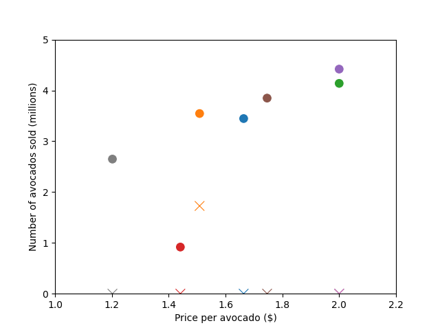
The circles represent sales quantity and the cross markers represent the wasted quantity.
We have shown how to model the price and supply optimization problem with Gurobi Machine Learning. In the Gurobi modeling examples notebook more analysis of the solutions this model can give is done interactively. Be sure to take look at it.
Copyright © 2023-2026 Gurobi Optimization, LLC
Total running time of the script: (0 minutes 0.690 seconds)