Note
Go to the end to download the full example code.
Surrogate Models
Some industrial applications require modeling complex processes that can result either in highly nonlinear functions or functions defined by a simulation process. In those contexts, optimization solvers often struggle. The reason may be that relaxations of the nonlinear functions are not good enough to make the solver prove an acceptable bound in a reasonable amount of time. Another issue may be that the solver is not able to represent the functions.
An approach that has been proposed in the literature is to approximate the problematic nonlinear functions via neural networks with ReLU activation and use MIP technology to solve the constructed approximation (see e.g. Heneao Maravelias 2011, Schweitdmann et.al. 2022). This use of neural networks can be motivated by their ability to provide a universal approximation (see e.g. Lu et.al. 2017). This use of ML models to replace complex processes is often referred to as surrogate models.
In the following example, we approximate a nonlinear function via
Scikit-learn MLPRegressor and then solve an optimization problem
that uses the approximation of the nonlinear function with Gurobi.
The purpose of this example is solely illustrative and doesn’t relate to any particular application.
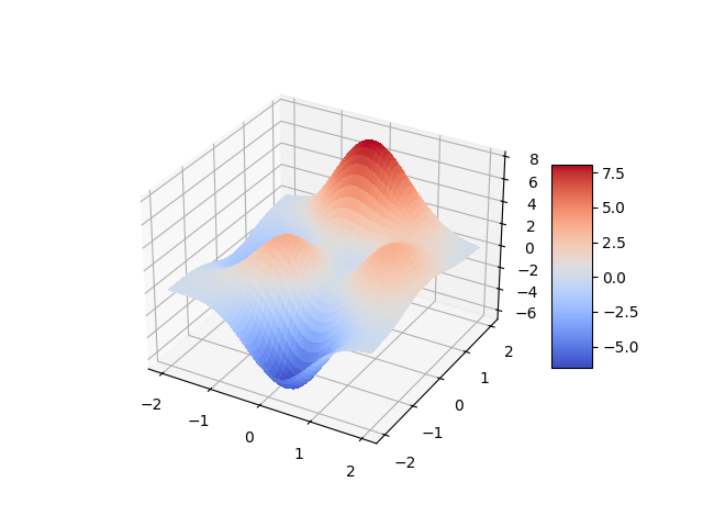
The function we approximate is the 2D peaks function.
The function is given as
In this example, we want to find the minimum of \(f\) over the interval \([-2, 2]^2\):
The global minimum of this problem can be found numerically to have value \(-6.55113\) at the point \((0.2283, -1.6256)\).
Here to find this minimum of \(f\), we approximate \(f(x)\) through a neural network function \(g(x)\) to obtain a MIP and solve
First import the necessary packages. Before applying the neural network,
we do a preprocessing to extract polynomial features of degree 2.
Hopefully this will help us to approximate the smooth function. Besides,
gurobipy, numpy and the appropriate sklearn objects, we also
use matplotlib to plot the function, and its approximation.
import gurobipy as gp
import numpy as np
from gurobipy import GRB
from matplotlib import cm
from matplotlib import pyplot as plt
from sklearn import metrics
from sklearn.neural_network import MLPRegressor
from sklearn.pipeline import make_pipeline
from sklearn.preprocessing import PolynomialFeatures

from gurobi_ml import add_predictor_constr
Define the nonlinear function of interest
We define the 2D peak function as a python function.
def peak2d(x1, x2):
    return (
        3 * (1 - x1) ** 2.0 * np.exp(-(x1**2) - (x2 + 1) ** 2)
        - 10 * (x1 / 5 - x1**3 - x2**5) * np.exp(-(x1**2) - x2**2)
        - 1 / 3 * np.exp(-((x1 + 1) ** 2) - x2**2)
    )
To train the neural network, we make a uniform sample of the domain of
the function in the region of interest using numpy’s arrange
function.
We then plot the function with matplotlib.
x1, x2 = np.meshgrid(np.arange(-2, 2, 0.01), np.arange(-2, 2, 0.01))
y = peak2d(x1, x2)

fig, ax = plt.subplots(subplot_kw={"projection": "3d"})
# Plot the surface.
surf = ax.plot_surface(x1, x2, y, cmap=cm.coolwarm, linewidth=0.01, antialiased=False)
# Add a color bar which maps values to colors.
fig.colorbar(surf, shrink=0.5, aspect=5)
plt.show()
Approximate the function
To fit a model, we need to reshape our data. We concatenate the values
of x1 and x2 in an array X and make y one dimensional.
X = np.concatenate([x1.ravel().reshape(-1, 1), x2.ravel().reshape(-1, 1)], axis=1)
y = y.ravel()
To approximate the function, we use a Pipeline with polynomial
features and a neural-network regressor. We do a relatively small
neural-network.
# Run our regression
layers = [30] * 2
regression = MLPRegressor(hidden_layer_sizes=layers, activation="relu")
pipe = make_pipeline(PolynomialFeatures(), regression)
pipe.fit(X=X, y=y)
To test the accuracy of the approximation, we take a random sample of points, and we print the \(R^2\) value and the maximal error.
X_test = np.random.random((100, 2)) * 4 - 2

r2_score = metrics.r2_score(peak2d(X_test[:, 0], X_test[:, 1]), pipe.predict(X_test))
max_error = metrics.max_error(peak2d(X_test[:, 0], X_test[:, 1]), pipe.predict(X_test))
print("R2 error {}, maximal error {}".format(r2_score, max_error))
R2 error 0.9997599656840667, maximal error 0.0789578285216539
While the \(R^2\) value is good, the maximal error is quite high. For the purpose of this example we still deem it acceptable. We plot the function.
fig, ax = plt.subplots(subplot_kw={"projection": "3d"})
# Plot the surface.
surf = ax.plot_surface(
    x1,
    x2,
    pipe.predict(X).reshape(x1.shape),
    cmap=cm.coolwarm,
    linewidth=0.01,
    antialiased=False,
)
# Add a color bar which maps values to colors.
fig.colorbar(surf, shrink=0.5, aspect=5)
plt.show()

Visually, the approximation looks close enough to the original function.
Build and Solve the Optimization Model
We now turn to the optimization model. For this model we want to find
the minimal value of y_approx which is the approximation given by
our pipeline on the interval.
Note that in this simple example, we don’t use matrix variables but regular Gurobi variables instead.
m = gp.Model()

x = m.addVars(2, lb=-2, ub=2, name="x")
y_approx = m.addVar(lb=-GRB.INFINITY, name="y")

m.setObjective(y_approx, gp.GRB.MINIMIZE)

# add "surrogate constraint"
pred_constr = add_predictor_constr(m, pipe, x, y_approx)

pred_constr.print_stats()
Restricted license - for non-production use only - expires 2026-11-23
Warning for adding constraints: zero or small (< 1e-13) coefficients, ignored
Model for pipe:
126 variables
61 constraints
6 quadratic constraints
60 general constraints
Input has shape (1, 2)
Output has shape (1, 1)

Pipeline has 2 steps:

--------------------------------------------------------------------------------
Step            Output Shape    Variables              Constraints
                                                Linear    Quadratic      General
================================================================================
poly_feat             (1, 6)            6            0            6            0

dense                (1, 30)           60           30            0           30 (relu)

dense0               (1, 30)           60           30            0           30 (relu)

dense1                (1, 1)            0            1            0            0


--------------------------------------------------------------------------------
Now call optimize. Since we use polynomial features the resulting
model is a non-convex quadratic problem. In Gurobi, we need to set the
parameter NonConvex to 2 to be able to solve it.
m.Params.TimeLimit = 20
m.Params.MIPGap = 0.1
m.Params.NonConvex = 2

m.optimize()
Set parameter TimeLimit to value 20
Set parameter MIPGap to value 0.1
Set parameter NonConvex to value 2
Gurobi Optimizer version 12.0.2 build v12.0.2rc0 (linux64 - "Ubuntu 24.04 LTS")

CPU model: Intel(R) Xeon(R) Platinum 8488C, instruction set [SSE2|AVX|AVX2|AVX512]
Thread count: 1 physical cores, 2 logical processors, using up to 2 threads

Non-default parameters:
TimeLimit  20
MIPGap  0.1
NonConvex  2

Optimize a model with 61 rows, 129 columns and 1074 nonzeros
Model fingerprint: 0x0f8df261
Model has 6 quadratic constraints
Model has 60 simple general constraints
  60 MAX
Variable types: 129 continuous, 0 integer (0 binary)
Coefficient statistics:
  Matrix range     [1e-04, 1e+00]
  QMatrix range    [1e+00, 1e+00]
  QLMatrix range   [1e+00, 1e+00]
  Objective range  [1e+00, 1e+00]
  Bounds range     [2e+00, 2e+00]
  RHS range        [2e-02, 7e-01]
  QRHS range       [1e+00, 1e+00]
Presolve added 74 rows and 11 columns
Presolve time: 0.00s
Presolved: 145 rows, 141 columns, 1230 nonzeros
Presolved model has 3 bilinear constraint(s)

Solving non-convex MIQCP

Variable types: 102 continuous, 39 integer (39 binary)

Root relaxation: objective -3.354291e+01, 179 iterations, 0.00 seconds (0.00 work units)

    Nodes    |    Current Node    |     Objective Bounds      |     Work
 Expl Unexpl |  Obj  Depth IntInf | Incumbent    BestBd   Gap | It/Node Time

     0     0  -33.54291    0   32          -  -33.54291      -     -    0s
     0     0  -30.37390    0   34          -  -30.37390      -     -    0s
     0     0  -30.27122    0   34          -  -30.27122      -     -    0s
     0     0  -26.76688    0   36          -  -26.76688      -     -    0s
     0     0  -25.92824    0   36          -  -25.92824      -     -    0s
     0     0  -25.92824    0   34          -  -25.92824      -     -    0s
     0     0  -25.92824    0   36          -  -25.92824      -     -    0s
     0     0  -25.77816    0   37          -  -25.77816      -     -    0s
     0     0  -25.71465    0   37          -  -25.71465      -     -    0s
     0     0  -25.35142    0   38          -  -25.35142      -     -    0s
     0     0  -25.30133    0   40          -  -25.30133      -     -    0s
     0     0  -24.94786    0   38          -  -24.94786      -     -    0s
     0     0  -24.87296    0   38          -  -24.87296      -     -    0s
     0     0  -24.72631    0   38          -  -24.72631      -     -    0s
     0     0  -24.61856    0   40          -  -24.61856      -     -    0s
     0     0  -24.36563    0   39          -  -24.36563      -     -    0s
     0     0  -24.34033    0   39          -  -24.34033      -     -    0s
     0     0  -24.03320    0   39          -  -24.03320      -     -    0s
     0     0  -23.97803    0   40          -  -23.97803      -     -    0s
     0     0  -23.60849    0   40          -  -23.60849      -     -    0s
     0     0  -23.50894    0   40          -  -23.50894      -     -    0s
     0     0  -23.36378    0   40          -  -23.36378      -     -    0s
     0     0  -23.34618    0   40          -  -23.34618      -     -    0s
     0     0  -23.28353    0   40          -  -23.28353      -     -    0s
     0     0  -23.25356    0   40          -  -23.25356      -     -    0s
     0     0  -23.10769    0   39          -  -23.10769      -     -    0s
     0     0  -23.04158    0   42          -  -23.04158      -     -    0s
     0     0  -22.91744    0   38          -  -22.91744      -     -    0s
     0     0  -22.89538    0   41          -  -22.89538      -     -    0s
     0     0  -22.79919    0   42          -  -22.79919      -     -    0s
     0     0  -22.79580    0   41          -  -22.79580      -     -    0s
     0     0  -22.59423    0   41          -  -22.59423      -     -    0s
     0     0  -22.56781    0   41          -  -22.56781      -     -    0s
     0     0  -22.51379    0   42          -  -22.51379      -     -    0s
     0     0  -22.50873    0   42          -  -22.50873      -     -    0s
     0     0  -22.46203    0   41          -  -22.46203      -     -    0s
     0     0  -22.46086    0   41          -  -22.46086      -     -    0s
H    0     0                       1.3860598  -22.46086  1720%     -    0s
     0     2  -22.44844    0   41    1.38606  -22.44844  1720%     -    0s
H   27    25                       0.8640185  -21.29174  2564%  38.4    0s
H   27    25                       0.8640162  -21.29174  2564%  38.4    0s
H  190   108                      -1.1601823  -18.24076  1472%  17.3    0s
*  205   107              39      -1.1767622  -18.24076  1450%  16.2    0s
H  239   125                      -1.1767640  -17.88540  1420%  15.8    0s
H  271    98                      -4.8751196  -17.50454   259%  16.3    0s
H  298    95                      -5.4925581  -15.67719   185%  16.7    0s
H  352    85                      -6.4847774  -14.75545   128%  16.7    0s
H  379    97                      -6.5663058  -14.75545   125%  16.2    0s
H  616    42                      -6.5671530   -8.30758  26.5%  18.2    0s

Cutting planes:
  Gomory: 4
  Cover: 1
  Implied bound: 37
  MIR: 118
  Flow cover: 37
  RLT: 1

Explored 652 nodes (13140 simplex iterations) in 0.61 seconds (0.60 work units)
Thread count was 2 (of 2 available processors)

Solution count 10: -6.56715 -6.56631 -6.48478 ... 1.38606

Optimal solution found (tolerance 1.00e-01)
Best objective -6.567153006392e+00, best bound -7.197651864409e+00, gap 9.6008%
After solving the model, we check the error in the estimate of the Gurobi solution.
print(
    "Maximum error in approximating the regression {:.6}".format(
        np.max(pred_constr.get_error())
    )
)
Maximum error in approximating the regression 4.66266e-06
Finally, we look at the solution and the objective value found.
print(
    f"solution point of the approximated problem ({x[0].X:.4}, {x[1].X:.4}), "
    + f"objective value {m.ObjVal}."
)
print(
    f"Function value at the solution point {peak2d(x[0].X, x[1].X)} error {abs(peak2d(x[0].X, x[1].X) - m.ObjVal)}."
)
solution point of the approximated problem (0.2399, -1.582), objective value -6.567153006392107.
Function value at the solution point -6.523933894771595 error 0.04321911162051162.
The difference between the function and the approximation at the computed solution point is noticeable, but the point we found is reasonably close to the actual global minimum. Depending on the use case this might be deemed acceptable. Of course, training a larger network should result in a better approximation.
Copyright © 2023 Gurobi Optimization, LLC
Total running time of the script: (0 minutes 5.391 seconds)