Note
Go to the end to download the full example code.
Adversarial Machine Learning
In this example, we show how to use Gurobi Machine Learning to construct an adversarial example for a trained neural network.
We use the MNIST handwritten digit database (http://yann.lecun.com/exdb/mnist/) for this example.
For this problem, we are given a trained neural network and one well classified example \(\bar x\). Our goal is to construct another example \(x\) close to \(\bar x\) that is classified with a different label.
For the hand digit recognition problem, the input is a grayscale image of \(28 \times 28\) (\(=784\)) pixels and the output is a vector of length 10 (each entry corresponding to a digit). We denote the output vector by \(y\). The image is classified according to the largest entry of \(y\).
For the training example, assume that coordinate \(l\) of the output vector is the one with the largest value giving the correct label. We pick a coordinate corresponding to another label, denoted \(w\), and we want the difference between \(y_w - y_l\) to be as large as possible.
If we can find a solution where this difference is positive, then \(x\) is a counter-example receiving a different label. If instead we can show that the difference is never positive, no such example exists.
Here, we use the \(l_1-\) norm \(|| x - \bar x||_1\) to define the neighborhood with its size defined by a fixed parameter \(\delta\):
Denoting by \(g\) the prediction function of the neural network, the full optimization model reads:
Note that our model is inspired by Fischet al. (2018).
Imports and loading data
First, we import the required packages for this example.
In addition to the usual packages, we will need matplotlib to plot
the digits, and joblib to load a pre-trained network and part of the
training data.
Note that from the gurobi_ml package we need to use directly the
add_mlp_regressor_constr function for reasons that will be clarified
later.
import gurobipy as gp
import numpy as np
from joblib import load
from matplotlib import pyplot as plt

from gurobi_ml.sklearn import add_mlp_regressor_constr
We load a neural network that was pre-trained with Scikit-learn’s MLPRegressor. The network is small (2 hidden layers of 50 neurons), finding a counter example shouldn’t be too difficult.
We also load the first 100 training examples of the MNIST dataset that we saved to avoid having to reload the full data set.
# Load the trained network and the examples
mnist_data = load("../../tests/predictors/mnist__mlpclassifier.joblib")
nn = mnist_data["predictor"]
X = mnist_data["data"]
Choose an example and set labels
Now we choose an example. Here we chose arbitrarily example 26. We plot
the example and verify if it is well predicted by calling the
predict function.
# Choose an example
exampleno = 26
example = X[exampleno : exampleno + 1, :]

plt.imshow(example.reshape((28, 28)), cmap="gray")

print(f"Predicted label {nn.predict(example)}")
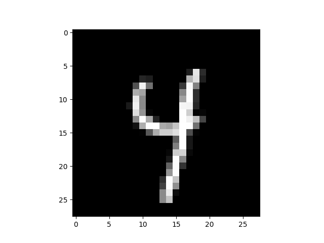
Predicted label ['4']
To set up the objective function of the optimization model, we also need to find a wrong label.
We use predict_proba to get the weight given by the neural network
to each label. We then use numpy’s argsort function to get the
labels sorted by their weight. The right label is then the last element
in the list, and we pick the next to last element as the wrong label.
ex_prob = nn.predict_proba(example)
sorted_labels = np.argsort(ex_prob)[0]
right_label = sorted_labels[-1]
wrong_label = sorted_labels[-2]
Building the optimization model
Now all the data is gathered, and we proceed to building the optimization model.
We create a matrix variable x corresponding to the new input of the
neural network we want to compute and a y matrix variable for the
output of the neural network. Those variables should have respectively
the shape of the example we picked and the shape of the return value of
predict_proba.
We need additional variables to model the \(l1-\)norm constraint.
Namely, for each pixel in the image, we need to measure the absolute
difference between \(x\) and \(\bar x\). The corresponding
matrix variable has the same shape as x.
We set the objective which is to maximize the difference between the wrong label and the right label.
m = gp.Model()
delta = 5

x = m.addMVar(example.shape, lb=0.0, ub=1.0, name="x")
y = m.addMVar(ex_prob.shape, lb=-gp.GRB.INFINITY, name="y")

abs_diff = m.addMVar(example.shape, lb=0, ub=1, name="abs_diff")

m.setObjective(y[0, wrong_label] - y[0, right_label], gp.GRB.MAXIMIZE)
The \(l1-\)norm constraint is formulated with:
With \(\eta\) denoting the absdiff variables.
Those constraints are naturally expressed with Gurobi’s Matrix API.
# Bound on the distance to example in norm-1
m.addConstr(abs_diff >= x - example)
m.addConstr(abs_diff >= -x + example)
m.addConstr(abs_diff.sum() <= delta)

# Update the model
m.update()
Finally, we insert the neural network in the gurobipy model to link
x and y.
Note that this case is not as straightforward as others. The reason is
that the neural network is trained for classification with a
"softmax" activation in the last layer. But in this model we are
using the network without activation in the last layer.
For this reason, we change manually the last layer activation before adding the network to the Gurobi model.
Also, we use the function
add_mlp_regressor_constr.
directly. The network being actually for classification (i.e. of type
MLPClassifier) the
add_predictor_constr.
function would not handle it automatically.
In the output, there is a warning about adding constraints with very small coefficients that are ignored. Neural-networks often contain very small coefficients in their expressions. Any coefficient with an absolute value smaller than \(10^{-13}\) is ignored by Gurobi. This may result in slightly different predicted values but should be negligible.
# Change last layer activation to identity
nn.out_activation_ = "identity"
# Code to add the neural network to the constraints
pred_constr = add_mlp_regressor_constr(m, nn, x, y)

# Restore activation
nn.out_activation_ = "softmax"
Warning for adding constraints: zero or small (< 1e-13) coefficients, ignored
The model should be complete. We print the statistics of what was added to insert the neural network into the optimization model.
Model for mlpclassifier:
200 variables
110 constraints
100 general constraints
Input has shape (1, 784)
Output has shape (1, 10)

--------------------------------------------------------------------------------
Layer           Output Shape    Variables              Constraints
                                                Linear    Quadratic      General
================================================================================
dense                (1, 50)          100           50            0           50 (relu)

dense0               (1, 50)          100           50            0           50 (relu)

dense1               (1, 10)            0           10            0            0

--------------------------------------------------------------------------------
Solving the model
We now turn to solving the optimization model. Solving the adversarial problem, as we formulated it above, doesn’t actually require computing a provably optimal solution. Instead, we need to either:
find a feasible solution with a positive objective cost (i.e. a counter-example), or
prove that there is no solution of positive cost (i.e. no counter-example in the neighborhood exists).
We can use Gurobi parameters to limit the optimization to answer those questions: setting BestObjStop to 0.0 will stop the optimizer if a counter-example is found, setting BestBdStop to 0.0 will stop the optimization if the optimizer has shown there is no counter-example.
We set the two parameters and optimize.
m.Params.BestBdStop = 0.0
m.Params.BestObjStop = 0.0
m.optimize()
Set parameter BestBdStop to value 0
Set parameter BestObjStop to value 0
Gurobi Optimizer version 12.0.2 build v12.0.2rc0 (linux64 - "Ubuntu 24.04 LTS")

CPU model: AMD EPYC 9R14, instruction set [SSE2|AVX|AVX2|AVX512]
Thread count: 2 physical cores, 2 logical processors, using up to 2 threads

Non-default parameters:
BestObjStop  0
BestBdStop  0

Optimize a model with 1679 rows, 1778 columns and 41839 nonzeros
Model fingerprint: 0xddfd4fc0
Model has 100 simple general constraints
  100 MAX
Variable types: 1778 continuous, 0 integer (0 binary)
Coefficient statistics:
  Matrix range     [1e-13, 2e+00]
  Objective range  [1e+00, 1e+00]
  Bounds range     [1e+00, 1e+00]
  RHS range        [2e-03, 5e+00]
Presolve removed 1236 rows and 720 columns
Presolve time: 0.09s
Presolved: 443 rows, 1058 columns, 38220 nonzeros
Variable types: 977 continuous, 81 integer (80 binary)

Root relaxation: objective 3.111795e+03, 313 iterations, 0.01 seconds (0.01 work units)

    Nodes    |    Current Node    |     Objective Bounds      |     Work
 Expl Unexpl |  Obj  Depth IntInf | Incumbent    BestBd   Gap | It/Node Time

     0     0 3111.79520    0   59          - 3111.79520      -     -    0s
     0     0 2937.07719    0   61          - 2937.07719      -     -    0s
     0     0 2934.15827    0   61          - 2934.15827      -     -    0s
     0     0 2804.51130    0   64          - 2804.51130      -     -    0s
     0     0 2788.91989    0   63          - 2788.91989      -     -    0s
     0     0 2788.62223    0   62          - 2788.62223      -     -    0s
     0     0 2630.10634    0   64          - 2630.10634      -     -    0s
     0     0 2604.91156    0   64          - 2604.91156      -     -    0s
     0     0 2604.58610    0   65          - 2604.58610      -     -    0s
     0     0 2604.57796    0   65          - 2604.57796      -     -    0s
     0     0 2304.57171    0   67          - 2304.57171      -     -    0s
     0     0 2258.36165    0   67          - 2258.36165      -     -    0s
     0     0 2253.88264    0   68          - 2253.88264      -     -    0s
     0     0 2253.24879    0   68          - 2253.24879      -     -    0s
     0     0 2253.09634    0   69          - 2253.09634      -     -    0s
     0     0 1841.97313    0   67          - 1841.97313      -     -    0s
     0     0 1807.67392    0   65          - 1807.67392      -     -    0s
     0     0 1802.34823    0   66          - 1802.34823      -     -    0s
     0     0 1801.39566    0   67          - 1801.39566      -     -    0s
     0     0 1801.26463    0   67          - 1801.26463      -     -    0s
     0     0 1540.48985    0   72          - 1540.48985      -     -    0s
     0     0 1458.49684    0   73          - 1458.49684      -     -    0s
     0     0 1452.96649    0   72          - 1452.96649      -     -    0s
     0     0 1450.73173    0   73          - 1450.73173      -     -    0s
     0     0 1450.48261    0   74          - 1450.48261      -     -    0s
     0     0 1320.15917    0   72          - 1320.15917      -     -    0s
     0     0 1291.41254    0   74          - 1291.41254      -     -    0s
     0     0 1285.41869    0   72          - 1285.41869      -     -    0s
     0     0 1284.75019    0   72          - 1284.75019      -     -    0s
     0     0 1199.38238    0   77          - 1199.38238      -     -    0s
     0     0 1190.68898    0   78          - 1190.68898      -     -    0s
     0     0 1189.57287    0   77          - 1189.57287      -     -    0s
     0     0 1135.16234    0   75          - 1135.16234      -     -    0s
     0     0 1110.75775    0   75          - 1110.75775      -     -    0s
     0     0 1109.26295    0   75          - 1109.26295      -     -    0s
     0     0  957.95470    0   74          -  957.95470      -     -    0s
     0     0  946.27581    0   75          -  946.27581      -     -    0s
     0     0  945.80707    0   74          -  945.80707      -     -    0s
     0     0  887.91010    0   74          -  887.91010      -     -    0s
     0     0  883.74553    0   77          -  883.74553      -     -    0s
     0     0  882.54428    0   75          -  882.54428      -     -    0s
     0     0  838.95187    0   75          -  838.95187      -     -    1s
     0     0  836.91654    0   75          -  836.91654      -     -    1s
     0     0  810.71694    0   75          -  810.71694      -     -    1s
     0     0  807.29012    0   76          -  807.29012      -     -    1s
     0     0  806.31233    0   76          -  806.31233      -     -    1s
     0     0  782.06027    0   74          -  782.06027      -     -    1s
     0     0  780.68826    0   76          -  780.68826      -     -    1s
     0     0  768.08048    0   76          -  768.08048      -     -    1s
     0     0  767.68093    0   76          -  767.68093      -     -    1s
     0     2  767.68093    0   76          -  767.68093      -     -    1s
   851   703   31.73183   36   76          -  284.48812      -  36.5    5s
   895   735  177.95133   14   71          -  177.95133      -  42.5   10s
H  910   709                      -1.8100471   64.76664  3678%  43.8   12s
* 1077   724              99       1.8377948   58.58990  3088%  43.8   13s

Cutting planes:
  MIR: 32
  Flow cover: 43

Explored 1088 nodes (51998 simplex iterations) in 13.44 seconds (28.21 work units)
Thread count was 2 (of 2 available processors)

Solution count 2: 1.83779 -1.81005

Optimization achieved user objective limit
Best objective 1.837794836162e+00, best bound 5.857562249726e+01, gap 3087.2776%
Results
Normally, for the example and \(\delta\) we chose, a counter example that gets the wrong label is found. We finish this notebook by plotting the counter example and printing how it is classified by the neural network.
plt.imshow(x.X.reshape((28, 28)), cmap="gray")

print(f"Solution is classified as {nn.predict(x.X)}")
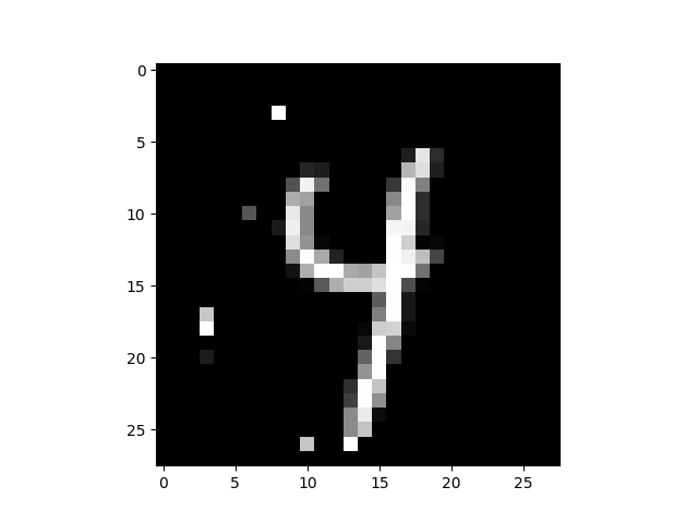
Solution is classified as ['9']
Copyright © 2023 Gurobi Optimization, LLC
Total running time of the script: (0 minutes 13.527 seconds)