Note

Go to the end to download the full example code.

Surrogate Models¶

Some industrial applications require modeling complex processes that can result either in highly nonlinear functions or functions defined by a simulation process. In those contexts, optimization solvers often struggle. The reason may be that relaxations of the nonlinear functions are not good enough to make the solver prove an acceptable bound in a reasonable amount of time. Another issue may be that the solver is not able to represent the functions.

An approach that has been proposed in the literature is to approximate the problematic nonlinear functions via neural networks with ReLU activation and use MIP technology to solve the constructed approximation (see e.g. Heneao Maravelias 2011, Schweitdmann et.al. 2022). This use of neural networks can be motivated by their ability to provide a universal approximation (see e.g. Lu et.al. 2017). This use of ML models to replace complex processes is often referred to as surrogate models.

In the following example, we approximate a nonlinear function via Scikit-learn MLPRegressor and then solve an optimization problem that uses the approximation of the nonlinear function with Gurobi.

The purpose of this example is solely illustrative and doesn’t relate to any particular application.

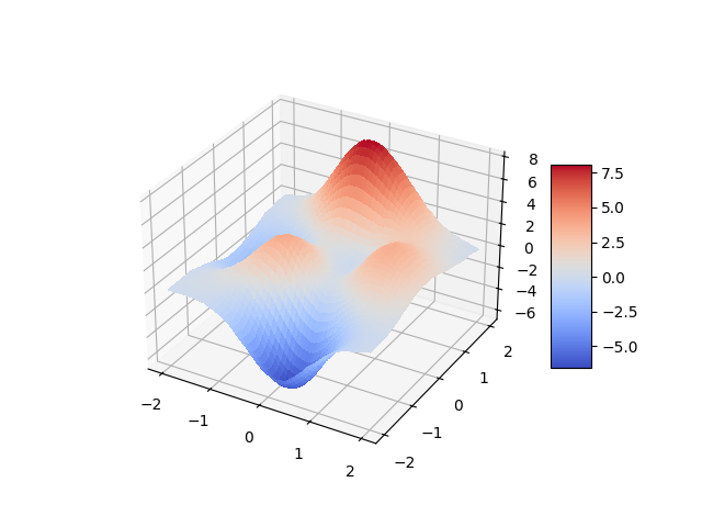
The function we approximate is the 2D peaks function.

The function is given as

\[\begin{split} \begin{aligned} f(x) = & 3 \cdot (1-x_1)^2 \cdot \exp(-x_1^2 - (x_2+1)^2) - \\ & 10 \cdot (\frac{x_1}{5} - x_1^3 - x_2^5) \cdot \exp(-x_1^2 - x_2^2) - \\ & \frac{1}{3} \cdot \exp(-(x_1+1)^2 - x_2^2). \end{aligned}\end{split}\]

In this example, we want to find the minimum of \(f\) over the interval \([-2, 2]^2\):

\[y = \min \{f(x) : x \in [-2,2]^2\}.\]

The global minimum of this problem can be found numerically to have value \(-6.55113\) at the point \((0.2283, -1.6256)\).

Here to find this minimum of \(f\), we approximate \(f(x)\) through a neural network function \(g(x)\) to obtain a MIP and solve

\[\hat y = \min \{g(x) : x \in [-2,2]^2\} \approx y.\]

First import the necessary packages. Before applying the neural network, we do a preprocessing to extract polynomial features of degree 2. Hopefully this will help us to approximate the smooth function. Besides, gurobipy, numpy and the appropriate sklearn objects, we also use matplotlib to plot the function, and its approximation.

import gurobipy as gp
import numpy as np
from gurobipy import GRB
from matplotlib import cm
from matplotlib import pyplot as plt
from sklearn import metrics
from sklearn.neural_network import MLPRegressor
from sklearn.pipeline import make_pipeline
from sklearn.preprocessing import PolynomialFeatures

from gurobi_ml import add_predictor_constr

Define the nonlinear function of interest¶

We define the 2D peak function as a python function.

def peak2d(x1, x2):
    return (
        3 * (1 - x1) ** 2.0 * np.exp(-(x1**2) - (x2 + 1) ** 2)
        - 10 * (x1 / 5 - x1**3 - x2**5) * np.exp(-(x1**2) - x2**2)
        - 1 / 3 * np.exp(-((x1 + 1) ** 2) - x2**2)
    )

To train the neural network, we make a uniform sample of the domain of the function in the region of interest using numpy’s arrange function.

We then plot the function with matplotlib.

x1, x2 = np.meshgrid(np.arange(-2, 2, 0.01), np.arange(-2, 2, 0.01))
y = peak2d(x1, x2)

fig, ax = plt.subplots(subplot_kw={"projection": "3d"})
# Plot the surface.
surf = ax.plot_surface(x1, x2, y, cmap=cm.coolwarm, linewidth=0.01, antialiased=False)
# Add a color bar which maps values to colors.
fig.colorbar(surf, shrink=0.5, aspect=5)
plt.show()

Approximate the function¶

To fit a model, we need to reshape our data. We concatenate the values of x1 and x2 in an array X and make y one dimensional.

X = np.concatenate([x1.ravel().reshape(-1, 1), x2.ravel().reshape(-1, 1)], axis=1)
y = y.ravel()

To approximate the function, we use a Pipeline with polynomial features and a neural-network regressor. We do a relatively small neural-network.

# Run our regression
layers = [30] * 2
regression = MLPRegressor(hidden_layer_sizes=layers, activation="relu")
pipe = make_pipeline(PolynomialFeatures(), regression)
pipe.fit(X=X, y=y)

Pipeline(steps=[('polynomialfeatures', PolynomialFeatures()),
                ('mlpregressor', MLPRegressor(hidden_layer_sizes=[30, 30]))])

In a Jupyter environment, please rerun this cell to show the HTML representation or trust the notebook.
On GitHub, the HTML representation is unable to render, please try loading this page with nbviewer.org.

Pipeline

?Documentation for PipelineiFitted

Parameters

	steps steps: list of tuples List of (name of step, estimator) tuples that are to be chained in sequential order. To be compatible with the scikit-learn API, all steps must define `fit`. All non-last steps must also define `transform`. See :ref:`Combining Estimators <combining_estimators>` for more details.	[('polynomialfeatures', ...), ('mlpregressor', ...)]
	transform_input transform_input: list of str, default=None The names of the :term:`metadata` parameters that should be transformed by the pipeline before passing it to the step consuming it. This enables transforming some input arguments to ``fit`` (other than ``X``) to be transformed by the steps of the pipeline up to the step which requires them. Requirement is defined via :ref:`metadata routing <metadata_routing>`. For instance, this can be used to pass a validation set through the pipeline. You can only set this if metadata routing is enabled, which you can enable using ``sklearn.set_config(enable_metadata_routing=True)``. .. versionadded:: 1.6	None
	memory memory: str or object with the joblib.Memory interface, default=None Used to cache the fitted transformers of the pipeline. The last step will never be cached, even if it is a transformer. By default, no caching is performed. If a string is given, it is the path to the caching directory. Enabling caching triggers a clone of the transformers before fitting. Therefore, the transformer instance given to the pipeline cannot be inspected directly. Use the attribute ``named_steps`` or ``steps`` to inspect estimators within the pipeline. Caching the transformers is advantageous when fitting is time consuming. See :ref:`sphx_glr_auto_examples_neighbors_plot_caching_nearest_neighbors.py` for an example on how to enable caching.	None
	verbose verbose: bool, default=False If True, the time elapsed while fitting each step will be printed as it is completed.	False

Fitted attributes

Name	Type	Value
n_features_in_ n_features_in_: int Number of features seen during :term:`fit`. Only defined if the underlying first estimator in `steps` exposes such an attribute when fit. .. versionadded:: 0.24	int	2

PolynomialFeatures

?Documentation for PolynomialFeatures

Parameters

	degree degree: int or tuple (min_degree, max_degree), default=2 If a single int is given, it specifies the maximal degree of the polynomial features. If a tuple `(min_degree, max_degree)` is passed, then `min_degree` is the minimum and `max_degree` is the maximum polynomial degree of the generated features. Note that `min_degree=0` and `min_degree=1` are equivalent as outputting the degree zero term is determined by `include_bias`.	2
	interaction_only interaction_only: bool, default=False If `True`, only interaction features are produced: features that are products of at most `degree` distinct input features, i.e. terms with power of 2 or higher of the same input feature are excluded: - included: `x[0]`, `x[1]`, `x[0] * x[1]`, etc. - excluded: `x[0] 2`, `x[0] 2 * x[1]`, etc.	False
	include_bias include_bias: bool, default=True If `True` (default), then include a bias column, the feature in which all polynomial powers are zero (i.e. a column of ones - acts as an intercept term in a linear model).	True
	order order: {'C', 'F'}, default='C' Order of output array in the dense case. `'F'` order is faster to compute, but may slow down subsequent estimators. .. versionadded:: 0.21	'C'

Fitted attributes

Name	Type	Value
n_features_in_ n_features_in_: int Number of features seen during :term:`fit`. .. versionadded:: 0.24	int	2
n_output_features_ n_output_features_: int The total number of polynomial output features. The number of output features is computed by iterating over all suitably sized combinations of input features.	int	6
powers_ powers_: ndarray of shape (`n_output_features_`, `n_features_in_`) `powers_[i, j]` is the exponent of the jth input in the ith output.	ndarray[int64](6, 2)	[[0,0], [1,0], [0,1], [2,0], [1,1], [0,2]]

6 features

x0^2

x0 x1

x1^2

MLPRegressor

?Documentation for MLPRegressor

Parameters

	hidden_layer_sizes hidden_layer_sizes: array-like of shape(n_layers - 2,), default=(100,) The ith element represents the number of neurons in the ith hidden layer.	[30, 30]
	loss loss: {'squared_error', 'poisson'}, default='squared_error' The loss function to use when training the weights. Note that the "squared error" and "poisson" losses actually implement "half squares error" and "half poisson deviance" to simplify the computation of the gradient. Furthermore, the "poisson" loss internally uses a log-link (exponential as the output activation function) and requires ``y >= 0``. .. versionchanged:: 1.7 Added parameter `loss` and option 'poisson'.	'squared_error'
	activation activation: {'identity', 'logistic', 'tanh', 'relu'}, default='relu' Activation function for the hidden layer. - 'identity', no-op activation, useful to implement linear bottleneck, returns f(x) = x - 'logistic', the logistic sigmoid function, returns f(x) = 1 / (1 + exp(-x)). - 'tanh', the hyperbolic tan function, returns f(x) = tanh(x). - 'relu', the rectified linear unit function, returns f(x) = max(0, x)	'relu'
	solver solver: {'lbfgs', 'sgd', 'adam'}, default='adam' The solver for weight optimization. - 'lbfgs' is an optimizer in the family of quasi-Newton methods. - 'sgd' refers to stochastic gradient descent. - 'adam' refers to a stochastic gradient-based optimizer proposed by Kingma, Diederik, and Jimmy Ba For a comparison between Adam optimizer and SGD, see :ref:`sphx_glr_auto_examples_neural_networks_plot_mlp_training_curves.py`. Note: The default solver 'adam' works pretty well on relatively large datasets (with thousands of training samples or more) in terms of both training time and validation score. For small datasets, however, 'lbfgs' can converge faster and perform better.	'adam'
	alpha alpha: float, default=0.0001 Strength of the L2 regularization term. The L2 regularization term is divided by the sample size when added to the loss.	0.0001
	batch_size batch_size: int, default='auto' Size of minibatches for stochastic optimizers. If the solver is 'lbfgs', the regressor will not use minibatch. When set to "auto", `batch_size=min(200, n_samples)`.	'auto'
	learning_rate learning_rate: {'constant', 'invscaling', 'adaptive'}, default='constant' Learning rate schedule for weight updates. - 'constant' is a constant learning rate given by 'learning_rate_init'. - 'invscaling' gradually decreases the learning rate ``learning_rate_`` at each time step 't' using an inverse scaling exponent of 'power_t'. effective_learning_rate = learning_rate_init / pow(t, power_t) - 'adaptive' keeps the learning rate constant to 'learning_rate_init' as long as training loss keeps decreasing. Each time two consecutive epochs fail to decrease training loss by at least tol, or fail to increase validation score by at least tol if 'early_stopping' is on, the current learning rate is divided by 5. Only used when solver='sgd'.	'constant'
	learning_rate_init learning_rate_init: float, default=0.001 The initial learning rate used. It controls the step-size in updating the weights. Only used when solver='sgd' or 'adam'.	0.001
	power_t power_t: float, default=0.5 The exponent for inverse scaling learning rate. It is used in updating effective learning rate when the learning_rate is set to 'invscaling'. Only used when solver='sgd'.	0.5
	max_iter max_iter: int, default=200 Maximum number of iterations. The solver iterates until convergence (determined by 'tol') or this number of iterations. For stochastic solvers ('sgd', 'adam'), note that this determines the number of epochs (how many times each data point will be used), not the number of gradient steps.	200
	shuffle shuffle: bool, default=True Whether to shuffle samples in each iteration. Only used when solver='sgd' or 'adam'.	True
	random_state random_state: int, RandomState instance, default=None Determines random number generation for weights and bias initialization, train-test split if early stopping is used, and batch sampling when solver='sgd' or 'adam'. Pass an int for reproducible results across multiple function calls. See :term:`Glossary <random_state>`.	None
	tol tol: float, default=1e-4 Tolerance for the optimization. When the loss or score is not improving by at least ``tol`` for ``n_iter_no_change`` consecutive iterations, unless ``learning_rate`` is set to 'adaptive', convergence is considered to be reached and training stops.	0.0001
	verbose verbose: bool, default=False Whether to print progress messages to stdout.	False
	warm_start warm_start: bool, default=False When set to True, reuse the solution of the previous call to fit as initialization, otherwise, just erase the previous solution. See :term:`the Glossary <warm_start>`.	False
	momentum momentum: float, default=0.9 Momentum for gradient descent update. Should be between 0 and 1. Only used when solver='sgd'.	0.9
	nesterovs_momentum nesterovs_momentum: bool, default=True Whether to use Nesterov's momentum. Only used when solver='sgd' and momentum > 0.	True
	early_stopping early_stopping: bool, default=False Whether to use early stopping to terminate training when validation score is not improving. If set to True, it will automatically set aside ``validation_fraction`` of training data as validation and terminate training when validation score is not improving by at least ``tol`` for ``n_iter_no_change`` consecutive epochs. Only effective when solver='sgd' or 'adam'.	False
	validation_fraction validation_fraction: float, default=0.1 The proportion of training data to set aside as validation set for early stopping. Must be between 0 and 1. Only used if early_stopping is True.	0.1
	beta_1 beta_1: float, default=0.9 Exponential decay rate for estimates of first moment vector in adam, should be in [0, 1). Only used when solver='adam'.	0.9
	beta_2 beta_2: float, default=0.999 Exponential decay rate for estimates of second moment vector in adam, should be in [0, 1). Only used when solver='adam'.	0.999
	epsilon epsilon: float, default=1e-8 Value for numerical stability in adam. Only used when solver='adam'.	1e-08
	n_iter_no_change n_iter_no_change: int, default=10 Maximum number of epochs to not meet ``tol`` improvement. Only effective when solver='sgd' or 'adam'. .. versionadded:: 0.20	10
	max_fun max_fun: int, default=15000 Only used when solver='lbfgs'. Maximum number of function calls. The solver iterates until convergence (determined by ``tol``), number of iterations reaches max_iter, or this number of function calls. Note that number of function calls will be greater than or equal to the number of iterations for the MLPRegressor. .. versionadded:: 0.22	15000

Fitted attributes

Name	Type	Value
best_loss_ best_loss_: float The minimum loss reached by the solver throughout fitting. If `early_stopping=True`, this attribute is set to `None`. Refer to the `best_validation_score_` fitted attribute instead. Only accessible when solver='sgd' or 'adam'.	float64	0.0006823
best_validation_score_ best_validation_score_: float or None The best validation score (i.e. R2 score) that triggered the early stopping. Only available if `early_stopping=True`, otherwise the attribute is set to `None`. Only accessible when solver='sgd' or 'adam'.	NoneType	None
coefs_ coefs_: list of shape (n_layers - 1,) The ith element in the list represents the weight matrix corresponding to layer i.	list	[array([[-5.72...049913e-001]]), array([[ 6.78...517109e-001]]), array([[-0.49... 0.29927818]])]
intercepts_ intercepts_: list of shape (n_layers - 1,) The ith element in the list represents the bias vector corresponding to layer i + 1.	list	[array([-4.631...18792689e-01]), array([ 0.368... -0.01399331]), array([0.35807952])]
loss_ loss_: float The current loss computed with the loss function.	float64	0.0006823
loss_curve_ loss_curve_: list of shape (`n_iter_`,) Loss value evaluated at the end of each training step. The ith element in the list represents the loss at the ith iteration. Only accessible when solver='sgd' or 'adam'.	list	[np.float64(0....9255833314956), np.float64(0....8192395154642), np.float64(0....5951876629535), np.float64(0....8888200828221), ...]
n_features_in_ n_features_in_: int Number of features seen during :term:`fit`. .. versionadded:: 0.24	int	6
n_iter_ n_iter_: int The number of iterations the solver has run.	int	20
n_layers_ n_layers_: int Number of layers.	int	4
n_outputs_ n_outputs_: int Number of outputs.	int	1
out_activation_ out_activation_: str Name of the output activation function.	str	'id...ty'
t_ t_: int The number of training samples seen by the solver during fitting. Mathematically equals `n_iters * X.shape[0]`, it means `time_step` and it is used by optimizer's learning rate scheduler.	int	3200000
validation_scores_ validation_scores_: list of shape (`n_iter_`,) or None The score at each iteration on a held-out validation set. The score reported is the R2 score. Only available if `early_stopping=True`, otherwise the attribute is set to `None`. Only accessible when solver='sgd' or 'adam'.	NoneType	None

To test the accuracy of the approximation, we take a random sample of points, and we print the \(R^2\) value and the maximal error.

X_test = np.random.random((100, 2)) * 4 - 2

r2_score = metrics.r2_score(peak2d(X_test[:, 0], X_test[:, 1]), pipe.predict(X_test))
max_error = metrics.max_error(peak2d(X_test[:, 0], X_test[:, 1]), pipe.predict(X_test))
print(f"R2 error {r2_score}, maximal error {max_error}")

R2 error 0.9998048056414734, maximal error 0.09717518795032332

While the \(R^2\) value is good, the maximal error is quite high. For the purpose of this example we still deem it acceptable. We plot the function.

fig, ax = plt.subplots(subplot_kw={"projection": "3d"})
# Plot the surface.
surf = ax.plot_surface(
    x1,
    x2,
    pipe.predict(X).reshape(x1.shape),
    cmap=cm.coolwarm,
    linewidth=0.01,
    antialiased=False,
)
# Add a color bar which maps values to colors.
fig.colorbar(surf, shrink=0.5, aspect=5)
plt.show()

Visually, the approximation looks close enough to the original function.

Build and Solve the Optimization Model¶

We now turn to the optimization model. For this model we want to find the minimal value of y_approx which is the approximation given by our pipeline on the interval.

Note that in this simple example, we don’t use matrix variables but regular Gurobi variables instead.

m = gp.Model()

x = m.addVars(2, lb=-2, ub=2, name="x")
y_approx = m.addVar(lb=-GRB.INFINITY, name="y")

m.setObjective(y_approx, gp.GRB.MINIMIZE)

# add "surrogate constraint"
pred_constr = add_predictor_constr(m, pipe, x, y_approx)

pred_constr.print_stats()

Restricted license - for non-production use only - expires 2027-11-29
Warning for adding constraints: zero or small (< 1e-13) coefficients, ignored
Model for pipe:
126 variables
61 constraints
6 quadratic constraints
60 general constraints
Input has shape (1, 2)
Output has shape (1, 1)

Pipeline has 2 steps:

--------------------------------------------------------------------------------
Step            Output Shape    Variables              Constraints
                                                Linear    Quadratic      General
================================================================================
poly_feat             (1, 6)            6            0            6            0

dense                (1, 30)           60           30            0           30 (relu)

dense0               (1, 30)           60           30            0           30 (relu)

dense1                (1, 1)            0            1            0            0


--------------------------------------------------------------------------------

Now call optimize. Since we use polynomial features the resulting model is a non-convex quadratic problem. In Gurobi, we need to set the parameter NonConvex to 2 to be able to solve it.

m.Params.TimeLimit = 20
m.Params.MIPGap = 0.1
m.Params.NonConvex = 2

m.optimize()

Set parameter TimeLimit to value 20
Set parameter MIPGap to value 0.1
Set parameter NonConvex to value 2
Gurobi Optimizer version 13.0.2 build v13.0.2rc1 (linux64 - "Ubuntu 24.04 LTS")

CPU model: AMD EPYC 7R13 Processor, instruction set [SSE2|AVX|AVX2]
Thread count: 1 physical cores, 2 logical processors, using up to 2 threads

Non-default parameters:
TimeLimit  20
MIPGap  0.1
NonConvex  2

Optimize a model with 61 rows, 129 columns and 1096 nonzeros (Min)
Model fingerprint: 0x5d8af6f1
Model has 1 linear objective coefficients
Model has 6 quadratic constraints
Model has 60 simple general constraints
  60 MAX
Variable types: 129 continuous, 0 integer (0 binary)
Coefficient statistics:
  Matrix range     [3e-06, 2e+00]
  QMatrix range    [1e+00, 1e+00]
  QLMatrix range   [1e+00, 1e+00]
  Objective range  [1e+00, 1e+00]
  Bounds range     [2e+00, 2e+00]
  RHS range        [1e-04, 8e-01]
  QRHS range       [1e+00, 1e+00]

Presolve added 81 rows and 18 columns
Presolve time: 0.01s
Presolved: 152 rows, 148 columns, 1272 nonzeros
Presolved model has 3 bilinear constraint(s)

Solving non-convex MIQCP to global optimality

Variable types: 106 continuous, 42 integer (42 binary)

Root relaxation: objective -5.723325e+01, 175 iterations, 0.00 seconds (0.00 work units)

    Nodes    |    Current Node    |     Objective Bounds      |     Work
 Expl Unexpl |  Obj  Depth IntInf | Incumbent    BestBd   Gap | It/Node Time

     0     0  -57.23325    0   33          -  -57.23325      -     -    0s
     0     0  -57.01402    0   32          -  -57.01402      -     -    0s
     0     0  -49.73136    0   34          -  -49.73136      -     -    0s
     0     0  -46.14313    0   40          -  -46.14313      -     -    0s
H    0     0                      -6.1063420  -46.14265   656%     -    0s
     0     0  -46.06313    0   40   -6.10634  -46.06313   654%     -    0s
     0     0  -44.77374    0   37   -6.10634  -44.77374   633%     -    0s
     0     0  -44.45901    0   39   -6.10634  -44.45901   628%     -    0s
     0     0  -43.73383    0   39   -6.10634  -43.73383   616%     -    0s
     0     0  -43.56644    0   40   -6.10634  -43.56644   613%     -    0s
     0     0  -43.14445    0   41   -6.10634  -43.14445   607%     -    0s
     0     0  -43.03721    0   41   -6.10634  -43.03721   605%     -    0s
     0     0  -42.71507    0   40   -6.10634  -42.71507   600%     -    0s
     0     0  -42.61243    0   41   -6.10634  -42.61243   598%     -    0s
     0     0  -42.36073    0   41   -6.10634  -42.36073   594%     -    0s
     0     0  -42.36060    0   40   -6.10634  -42.36060   594%     -    0s
     0     0  -42.24039    0   40   -6.10634  -42.24039   592%     -    0s
     0     0  -41.86861    0   41   -6.10634  -41.86861   586%     -    0s
H    0     0                      -6.1063426  -41.84651   585%     -    0s
     0     0  -41.61093    0   41   -6.10634  -41.61093   581%     -    0s
     0     0  -41.22385    0   41   -6.10634  -41.22385   575%     -    0s
     0     0  -41.15022    0   42   -6.10634  -41.15022   574%     -    0s
     0     0  -41.04335    0   42   -6.10634  -41.04335   572%     -    0s
     0     0  -41.01327    0   40   -6.10634  -41.01327   572%     -    0s
     0     0  -40.86077    0   41   -6.10634  -40.86077   569%     -    0s
     0     0  -40.81240    0   42   -6.10634  -40.81240   568%     -    0s
     0     0  -40.73088    0   42   -6.10634  -40.73088   567%     -    0s
     0     0  -40.72553    0   41   -6.10634  -40.72553   567%     -    0s
     0     0  -40.59616    0   42   -6.10634  -40.59616   565%     -    0s
     0     0  -40.51622    0   41   -6.10634  -40.51622   564%     -    0s
     0     0  -40.38149    0   41   -6.10634  -40.38149   561%     -    0s
     0     0  -40.36030    0   41   -6.10634  -40.36030   561%     -    0s
     0     0  -40.27547    0   43   -6.10634  -40.27547   560%     -    0s
     0     0  -40.26452    0   43   -6.10634  -40.26452   559%     -    0s
     0     0  -40.26452    0   43   -6.10634  -40.26452   559%     -    0s
     0     2  -40.19956    0   43   -6.10634  -40.19956   558%     -    0s
H   11    11                      -6.1063431  -38.69687   534%  47.8    0s
H  724   413                      -6.3421264  -25.54135   303%  21.0    1s
H  731   398                      -6.4122439  -25.54135   298%  21.3    1s
H  739   380                      -6.4803553  -25.54135   294%  21.4    1s
H  878   388                      -6.4816922  -24.08123   272%  21.4    1s
H 5698   117                      -6.4816990   -8.15623  25.8%  18.9    4s
* 5716   121              48      -6.4816992   -8.15623  25.8%  18.9    4s
* 5718   121              49      -6.4816996   -8.15623  25.8%  18.9    4s

Cutting planes:
  Gomory: 10
  Cover: 2
  Implied bound: 17
  MIR: 117
  Flow cover: 60
  RLT: 1
  Relax-and-lift: 2

Explored 5838 nodes (110963 simplex iterations) in 4.15 seconds (4.27 work units)
Thread count was 2 (of 2 available processors)

Solution count 9: -6.4817 -6.4817 -6.4817 ... -6.10634

Optimal solution found (tolerance 1.00e-01)
Best objective -6.481699572118e+00, best bound -7.129647984870e+00, gap 9.9966%

After solving the model, we check the error in the estimate of the Gurobi solution.

print(
    "Maximum error in approximating the regression {:.6}".format(
        np.max(pred_constr.get_error())
    )
)

Maximum error in approximating the regression 1.17226e-06

Finally, we look at the solution and the objective value found.

print(
    f"solution point of the approximated problem ({x[0].X:.4}, {x[1].X:.4}), "
    + f"objective value {m.ObjVal}."
)
print(
    f"Function value at the solution point {peak2d(x[0].X, x[1].X)} error {abs(peak2d(x[0].X, x[1].X) - m.ObjVal)}."
)

solution point of the approximated problem (0.2263, -1.585), objective value -6.481699572118045.
Function value at the solution point -6.526737647552838 error 0.045038075434792546.

The difference between the function and the approximation at the computed solution point is noticeable, but the point we found is reasonably close to the actual global minimum. Depending on the use case this might be deemed acceptable. Of course, training a larger network should result in a better approximation.

Total running time of the script: (0 minutes 12.218 seconds)

Gallery generated by Sphinx-Gallery